Now that we've managed to capture a few mythological beasts and have quashed them inside our laptop for processing, we want a picture of it. After all, all of that work is a tall tale until you convince your friends with the pictorial evidence. This will make it easier to remember how to capture them the next time.
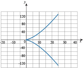
Much like scalar functions, when we draw vector functions, we get a much better idea of what they do and how they work. Like scalar functions, we begin the same way by plotting a table of values, graphing those values, and connecting the dots. See, math is like a game of connect-the-dots.
When graphing vector functions, we should be sure to know what values of the input variable we want to consider. Then we calculate the output values given by the vector function at those points.
Practice:
Sketch the vector function
f(t) = <t2,t3> for 0≤ t ≤ 5. | |
We make a table of values for x and y, going from t = 0 to t = 5: 
When we plot these points, we can see that they're lying along a curve: 
We connect the dots with that curve: 
| |
Sketch the vector function
f(t) = <t2,t3>
for -5≤ t ≤ 5. | |
We'll still have the part of the graph we found in the previous example, but now we need to figure out what happens for -5≤ t≤ 0. Make another table of values: 
Plotting these points and connecting them with a curve, we see that the graph of f(t) for -5≤ t ≤ 5 looks like this: 
| |
Sketch the vector function
f(t) = <t2,t3>.
| |
Since no bounds for t were given, this vector function is like the one in the previous exercise, but it keeps going. We can indicate this by drawing arrows on the
ends of the graph. | |
Sketch the vector function
f(t) =t, sin t>
for

- all real values of t
Answer
- Make a table, using values of t for which we can easily find the sine and cosine:
%%%%%%DATA ENTRY This data is in a table.
t & cost & sin t\hline0&1&0$\frac{π}{6}$&$\frac{\sqrt 3}{2}$&$\frac{1}{2}$$\frac{π}{4}$&$\frac{\sqrt 2}{2}$&$\frac{\sqrt2}{2}$$\frac{π}{3}$&$\frac{1}{2}$&$\frac{\sqrt3}{2}$$\frac{π}{2}$&0&1
0 ≤ t ≤ \frac{π}{2}These outline a quarter of a circle, which is what we find when we connect the dots:
PICTURE graph dots and the curve through themIf we replace t with θ, the coordinates (cos θ, sin θ) describe a point on the unit circle.Since $0 ≤ t ≤ \frac{π}{2}$, we get the portion of the unit circle where the angle goes from 0 to $\frac{π}{2}$.
- Since the coordinates are still describing the unit circle, this time we go around the whole unit circle:PICTURE: draw unit circle, label the point (1,0) with both t = 0 and t = 2π
- The coordinates are still describing the unit circle. The picture looks the same as the graph in part (B):PICTURE: vector funcs 6
However, since we're allowing ``all real values of <em>t" it's like we're traveling around the circle over and over. Every time <em>tem> is an integer multiple of 2π we pass through the point
(1,0). We'll talk more about this when we get to parametric equations.
Going up a dimension, here's a 3-D vector function:
f(t) = <cos t, sin t>.
For 0 < t < 4π, what does the graph of this function look like?
Answer
If we didn't have the third coordinate to worry about, this would be the unit circle again. Now it's like the unit circle, but each point is higher than the point before it:

It looks like a slinky or a blood-draining helical turn on a roller coaster.