When Velocity is Non-Negative
Again, let's assume we're cruising on the highway looking for some gas station nourishment. We could actually figure out the distance we've travelled by knowing our velocity and the time we spent searching.
We can only use the formula
distance = velocity × time
if velocity is constant on the time interval we're looking at. If we graph time on the horizontal axis and (constant) velocity on the vertical axis, we get this picture:
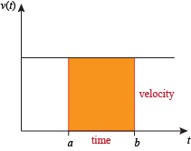
The area of this rectangle is velocity × time, which equals distance. The area of this rectangle also happens to be the definite integral of the (constant) velocity function on [a, b]. In symbols, when velocity is constant and positive on [a, b], the distance travelled from t = a to t = b is

Sample Problem
A car is traveling at v(t) = 60 mph. How far does the car travel in 20 minutes?
Answer.
20 minutes is one third of an hour, so

This is the area between the graph of the constant function v(t) = 60 and the t-axis on the interval  (or on any other interval of length
  hour).
If velocity isn't constant it's not clear how to apply the formula
distance = velocity × time.
What do we use for velocity? One approach is to pretend the velocity is constant: pick one reasonable value for the velocity and pretend that's the velocity for the whole time interval.
If we want to get a better estimate of distance travelled, we can split up the time interval into sub-intervals and pretend that velocity is constant on each sub-interval.
Sample Problem
Suppose Jen's velocity in mph was measured every ten minutes for one hour, and that her velocity was decreasing over that hour. The recorded values are shown in the table below. Estimate how far Jen travelled during the hour.

Answer.
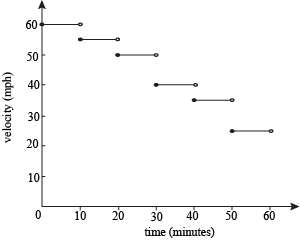
We don't know how fast Jen was going at every minute of the hour, but we can pretend that she was going 60 mph for the first ten minutes. Similarly, we can pretend she was going
55 mph from t = 10 to t = 20 minutes
50 mph from t = 20 to t = 30 minutes
40 mph from t = 30 to t = 40 minutes
35 mph from t = 40 to t = 50 minutes
25 mph from t = 50 to t = 60 minutes.
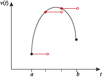
In real life her velocity would probably look something like this
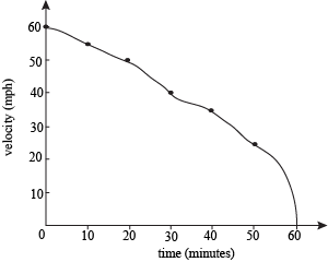
but to make the problem easier we're pretending her velocity looks like this:
Using the formula
distance = velocity × time
on each ten-minute sub-interval, we estimate that

Adding up the estimated distance for each 10-minute sub-interval, we estimate that over the full hour Jen travelled
10 + 9.2 + 8.3 + 6.7 + 5.8 + 4.2 = 44.2 miles.
On each sub-interval we're approximating Jen's velocity. She wasn't going 60 mph for all of the first ten minutes, so this answer is an estimate of how far Jen actually travelled.
In the example above, what we really did was use a left-hand sum with 6 sub-intervals to estimate

The upper limit of integration is 1 because the function v(t) expects t to be in hours.
When we use values of the velocity function and a right- or left-hand sum to approximate distance travelled from time t = a to time t = b, we're also approximating the integral of the velocity function on [a, b].
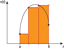
If the velocity function looks like this:
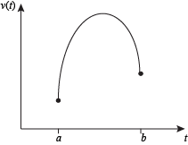
and we pretend it looks like this:
then the area of the rectangle on each sub-interval is our estimate of how far the cheetah or snail or whatever has travelled during that sub-interval.
As our velocity measurements get closer together, our estimates approach the real distance travelled. Our estimates are also approaching the integral of the velocity function. Since our estimates can't approach two different things, the real distance travelled and the integral of the velocity function must be the same. In symbols, when v(t) is non-negative,
