The Normal Distribution

Our humps, our humps, our lovely data humps. When we go out, collect data, and graph it, it often comes out looking something like this.

Well, we usually graph our data with a hot pink pen and doodle dragons and unicorns in the margins, but you get the idea. The data, those blue histogram bars, can be approximated by that slick curve. The most common values are in the middle of the distribution, and the absolute tippy-top of the curve, right there in the middle as well, equals the mean of the dataset.

What might we call such a curve? This is a rather popular distribution, so it has a lot of nicknames: the normal distribution is the most common, but it's also known as a Gaussian distribution or a bell-shaped curve. We think it's more hump shaped than bell shaped, but nobody asked for our opinion.

Beware the Eye of the Beholder

What is normal anyway? In real life, everybody has their quirks, oddities, and weird habits that mark them as strange in some aspect of their life. Trust us, we should know. People are just too different to pin down as strictly "normal" or "not normal." Except for that colony of clones living in the 'burbs.

In statistics, though, things are different. A dataset is normal when it follows a normal distribution. The most likely value is the mean in the middle, which also happens to equal the median and mode as well. Looks like they've made up since we last saw them. Also, a normal distribution is symmetric around the mean. Most of the data is close to the mean, and very small and very large results are equally rare.

If the data is skewed too much to the side, then the mean is offset from the middle of the curve. It might look normal to some people, but not to us.

But hey, what kinds of stuff will actually be normal when we graph them? Maybe not all the things, but still a lot. People's height is one example. Some people are Andre the Giant, some people are the 7 Dwarves, but most people are somewhere in the middle.

Other types of typically normal data include yearly rainfall amounts, some Wall Street stock indices, the velocity of molecules in an ideal gas, and all kinds of measurements in astronomy, biology, physics, medicine, and whatever other subject we might care to mention.

The normal distribution sure does get around.

A Bit Spread Out

A normal distribution is completely defined by its mean and standard deviation. They have no other secrets. The mean gives its location on the x-axis, while the standard deviation tells us the shape and spread of the curve. A large standard deviation makes the curve wide and kind a flat, while a small amount of spread makes it tall and narrow.

We can know more, though. A lot more. The mean and standard deviation tell us so much, in fact, that they're going to start their own advice hotline.

Sample Problem

On average, a dress from Ye Olde Dress Shoppe costs $1250. The standard deviation for dress prices is $200, and they follow a strict normal distribution pricing scheme. What range of prices covers 95% of their inventory?

Data in a normal distribution is on a tight leash. It can't go very far from the mean in the center of the distribution. The standard deviation gives us the length of the leash, according to a handy rule of thumb called the Empirical Rule:

• About 68% of the data are within 1 standard deviation of the mean. That's about ⅔ of the data.
• About 95% of the data are within 2 standard deviations of the mean. That's most of the data.
• About 99.7% of the data are within 3 standard deviations of the mean. Good golly that's a lot of data.

This is also called the 68-95-99.7 Rule, but that isn't very catchy. It's nice to look at, though.

The Shoppe keeps their prices normally distributed, so we know that 95% of their prices will be within 2 standard deviations above or below the mean.

$1250 ± $200

= $1050 and $1450

Those prices are a bit too rich for our blood. And it doesn't look like we'll have much luck finding a bargain sale. Only 5% of the dresses will be outside of that price range, and half of that 5% will be even more expensive. We'll stick to the shops without the extra 'pe' at the end.

The Shape of Things

The Empirical Rule only works when the data is actually normal. We'd think that would be obvious, but sometimes people just assume their data comes from a normal distribution without checking. So, don't do that.

A dataset's distribution can be skewed to the side, have multiple humps, or contain outliers. Unless we're told the data is normal, we have to check it out before we can use the Empirical Rule. Or any other rule that depends on having a normal distribution, we guess.

The Name of Things

The normal distribution has too many names already, and now we need to learn two more. The mean and standard deviation both have new symbols that they go by. The mean of a normal distribution is μ; that's called mu, and it's pronounced "mew." The standard deviation of a normal distribution is σ; we call that sigma, and we pronounce it "sigma."

These names only apply when we're talking about the mean and standard deviation of a normal distribution. When we are talking about our data, we'll still use x and s. Nothing else is changed about them. They just walk around in their funny costumes, and expect us not to laugh. It's very hard not to sometimes, though.

• Standard Normal Distribution

  So far we've been talking about the normal distribution, but that's like talking about the chocolate chip cookie recipe. There are a lot of ways to bake yummy cookies, and there are a lot of normal distributions out there.

  If the mean is 5 and the standard deviation is 10, that's a different distribution from x being 300 and s being 20. You don't even want to know what happens when the mean stops being polite and the standard deviation starts getting real.

  This is important when we want to find some probabilities associated with our data. Sometimes we get lucky, and we can use the Empirical Rule to find a probability. If 68% of the data falls within 1 standard deviation of the mean, that's the same as saying that there is a 68% chance of a random data point being from that region of the graph. But life isn't always that kind.

  What if our data is 0.5 standard deviations below the mean? Or 2.7 above it? Or, dare we even say it, what if we don't know how many standard deviations away from the mean we are? That may not sound like a big deal to you, but the idea makes any statistician quake in their square boots.

  The probability problem is solved by using the standard normal distribution. You wouldn't recognize it passing by on the street, but it's a very special normal distribution: it has a mean of 0 and a standard deviation of 1. When x = 1, we are 1 standard deviation above the mean of a standard normal distribution.

  

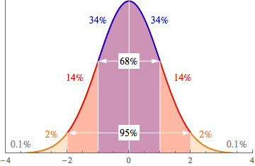
  Sound familiar? It's just like the graph of the Empirical Rule we've seen before. Take any normal distribution you care to imagine—if we move x standard deviations away from the mean, we can move x away from 0 on the standard normal distribution. It's like some wacky mirror-movement hijinks up in here.

  Our secret weapon for moving from a normal distribution to the standard normal one is the formula for the Z-score.

  

  So, if the number of hot dogs someone can eat in 10 minutes is normally distributed, with a mean of 5 and a standard deviation of 2, we can find Z for any number of hot dogs that we like. For Z = 2:

   

  = -1.5

  Only eating two hot dogs is kind of weak sauce. That's 1.5 standard deviations below the mean. The thing is, that's true for both the original distribution and the normal distribution. We expect better from a professional hot dog eater.

  We're going to use this fact to calculate some probabilities for the original distribution. Not the hot dog facts, the other one. But we're going to do that later. Not now. Now is the time on Shmoop when we dance.

• Using Z-Scores

  A normal distribution, a Z-score, and Shmoop walk into a classroom. The normal distribution and the Z-score say "ouch," while Shmoop gets to work on finding some probabilities.

  Sample Problem

  A dataset is normally distributed, with a mean of 177 and a standard deviation of 48. What is the probability of getting a result of 236 or greater?

  We like looking at pictures. What good is a scavenger hunt if we don't know what we're supposed to find?

  
  

  That shaded part under the curve will be the perfect spot for our picnic. It's also the same as the probability we are looking for. We can solve the problem and eat a peanut butter sandwich at the same time.

  We don't like this distribution, though. It has too many ants on it. We'd rather have the same spot on a standard normal distribution. That means finding the Z-score at 236.

  
  

  

  We can reword our question as, "What is the probability of getting a result greater than 1.23 standard deviations above the mean of a standard normal distribution?" Or, to put it in a real fancy, math-y way:

  Pr(x > 1.23) = ?

  We like this question a lot more, because someone else has already done the hardest work for us. We don't have to calculate the probability, we just have to track it down in a standard normal table. These things have hundreds of probabilities already calculated. The catch is that they can be a tad confusing to read at times. We'll walk through it nice and easy, don't worry.

  Here is an example of a standard standard normal table. We highly suggest clicking that link and following along with us. Notice the picture in the upper-right corner: the probabilities in the table are those to the right of Z, or Pr(x > Z). That's exactly what we need, so no complaints from us.

  To read the table, start on the left side and go down until you find the row next to "1.20." That's part of the Z-score we want to find. The other part is "0.03," and we can find that along the top part of the table.

  Z	0.02	0.03	0.04
  1.10	0.131357	0.129238	0.127143
  1.20	0.111233	0.109349	0.107488
  1.30	0.093418	0.091759	0.090123

  We travel along the row "1.20" and down the column "0.03" until our fingers run into each other. Where they meet is Pr(Z > 1.23), and that equals 0.109349. That equals the shaded-in part of the graph we've been looking for. Now if only this table could help us find our keys.

  Sample Problem

  A dataset is normally distributed, with a mean of 342 and a standard deviation of 74. What is the probability of getting a result of 166 or greater?

  Let's find the Z-score first, then we'll sketch what our probability looks like. Plugging into the Z-score formula we get:

  

  We put in our value first, then subtract the mean. Our result this time is a negative Z-score.

  
  

  This looks like a problem. Our table only has positive values for Z. What a busted piece of junk, only giving us half of what we need. We'd demand a refund, but we found it for free.

  All is not lost, though. Remember, the normal distribution is symmetric around the mean. The probability above positive Z will be equal to the probability below negative Z.

  
  

  That means there's a connection between 2.38, the number in the table, and -2.38, the number we need. A math connection, not a love connection, though. It is:

  Pr(x > 2.38) = Pr(x < -2.38)

  Watch those greater than and less than signs. It is super easy to mix up what they mean. That's why we're drawing so many graphs; they'll never give us up or let us down.

  The upshot here is that we don't have what we want yet. Using the standard normal table, we can find that Pr(x < -2.38) = Pr(x > 2.38) = 0.008656. That's the probability of getting a result below -2.38, but we want the probability above -2.38.

  The final piece of this puzzle is the fact that the total area underneath the curve of a normal distribution equals 1. The total probability of an event has to add up to 1, so that makes sense. It's useful for us, because it means:

  
  

  Setting up the problem we have:

  Pr(x > -2.38) = 1 – Pr(x < -2.38)

  = 1 – 0.008656

  = 0.991344

  And that's that. Our result matches what our first graph told us as well. Graphs: they stop us from making dumb mistakes.

  Sample Problem

  A dataset is normally distributed, with a mean of 70 and a standard deviation of 25. What is the probability of getting a result between 63 and 80?

  How good of a juggler are you? Because now we have two points to handle at once, and we want the probability between the two of them.

  We'll start by converting both of the points into Z-scores.

  

  

  

  Pr(-0.28 < x < 0.40) = ?

  We have an ice cream sandwich of a problem; we want to get at the good stuff in the middle. Our standard normal table only gives us the area to the right of each Z-score, but we can use a little subtraction wizardry to sort this out.

  
  

  Finding everything to the right of -0.28 will give us everything we need and some stuff we don't. What would we do with an extra kitchen sink anyway? If we subtract out all of the area to the right of 0.40, that will get rid of all the excess. We guess we can use the sink to cart off all the excess once we're done.

  Finding the area to the right of -0.28 is tricky, though, just like the last problem. Let's draw out the problem (in a good way) to solve this.

  
  

  Now we have the problem in a table-friendly form. It'll always use a coaster for its drinks, and it won't stick its feet up on the table either.

  Pr(x > -0.28) = 1 – Pr(x > 0.28)

  Find Pr(x > 0.28) by going down the rows of the table to "0.20," then across until you hit column "0.08."

  = 1 – 0.389739

  = 0.610261

  Hey hey, don't go and circle this as the answer. We want Pr(-0.28 < x < 0.40), so we still need to subtract out Pr(x > 0.40). At least the area above 0.40 is easy to find on the table.

  Pr(-0.28 < x < 0.40) = Pr(x > -0.28) – Pr(x > 0.40)

  = 0.610261 – 0.344578

  = 0.265683

  There we go, that's our answer. It's not quite as delicious as an ice cream sandwich, but still satisfying to have.

  The More Things Change, The More They're Different

  Here's one last word of warning for when we're finding probabilities with normal distributions. The table we gave you isn't the only kind out there. Instead of giving the probabilities to the right of the Z-scores, sometimes they'll give everything to the left. Or the area between 0 and Z. Even using a fancy graphing calculator won't save us from this confusion.

  So, cut through all that nonsense by always drawing lots of little graphs. If we can see what we're looking for, and what the table gives us, then there will be no problem-o. Plus it lets us practice our unicorn doodles.