The Wonderful World of Graphing
Finally, it's about time you were exposed to the wonderful world of graphing radical functions. Just like lines, parabolas, and trig functions, radicals have graphs, too. Here, we'll take just a couple minutes to introduce you to the parent graphs of a few of these delightful functions.

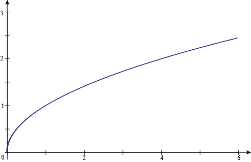
First on the list is . Since you can't take the square root of a negative number, the graph starts at (0, 0) and gets infinitely large as x continues to get bigger and bigger. That means that has a domain of all real numbers greater than or equal to 0. The range for this function is also all real numbers greater than or equal to 0. That's because the square root of a number can't be negative.
Oh, and quick reminder: a function's domain is the set of all its possible x-values (inputs). The range is just the function's set of possible y-values (output).
If you were to graph f (x) = ±√x, it would be exactly the same as the graph of f (x) = x2 rotated clockwise 90˚: a sideways parabola. Or as we like to say, it would be the same as f (x) = x2 if it were kicked in the head. Remember, violence is not the answer.

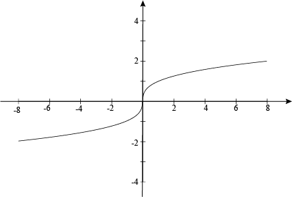
Next, it's none other than . This function is literally the inverse of f (x) = x3. This means that it's simply the graph of f (x) = x3 reflected across the line f (x) = x. Since you can put any x-value into this function, we say its domain is all real numbers. The range is also all real numbers, even though it might take a little bit longer for this particular function to climb to those gigantic numbers we associate with infinity.

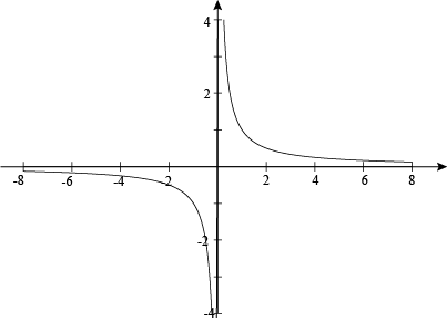
Since we also introduced you to negative exponents, we thought it would only be fair to give you some graphical knowledge as well. Meet , also known as f (x) = x -1. The graph of this kind fellow is known as a hyperbola. Since you can input any number except for 0, we say the domain is all real numbers except for 0. At x = 0, we've got a vertical asymptote. If this asymptote were anywhere else, it would be drawn with a dashed line. The function gets closer and closer to this imaginary line without ever quite getting there. Poor guy.
The range of is also all real numbers except for 0. At y = 0, we have what's called a horizontal asymptote. However, it's important to note that this horizontal asymptote is a way to describe the end behavior of the graph of . Unlike vertical asymptotes, which represent discontinuities or breaks in the function, the graph of a function can actually cross its horizontal asymptotes. Like here, in the graph of  .
.
True, this is a finer, more complicated point, but it is impressive knowledge to share on a first date.

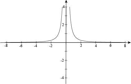
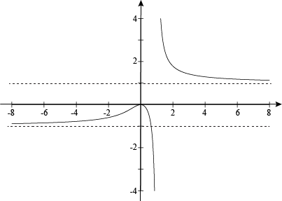
Last but not least, we humbly present . This graph looks a little something like  , but since the x is squared, all the output values are positive. This means that and have the same domain, but the range of is restricted to all real numbers greater than 0. Once again, there's a vertical asymptote at x = 0 and a horizontal asymptote at y = 0. Isn't that just the best word? Asymptote. Asymptote. It's almost as fun to say as Francisco.