Quantitative Genetics
Not Everything is Black or White: Quantitative Genetics
Most traits do not fall in discrete, qualitative categories (round or wrinkled, present or absent) but instead have a continuous, seemingly smooth spectrum of possible values. Height is a great example: people are not just short or tall, but can measure anywhere from 74.6 cm (2ft 5 in, the smallest man, He Ping Ping according to the Guinness Book of World Records) to 272 cm (8 ft 11.1 in, the tallest man, Robert Pershing Wadlow, also according to the Guinness Book of World Records). If we look at the distribution of height in men in the United States (based on measuring the height of 4,314 individuals), we find that most men measure around 176 cm (69.3 in), and that less than 5% measure 162.9 cm or less (≤ 64.1 in) or 188.4 cm or more (≥ 74.2 in) (McDowell, Fryar, Hirsch, & Ogden, 2005). If we plotted the height for all these people, we would find it makes a bell shape, where most individuals fall in the middle, with very short and very tall people at the ends, or tails.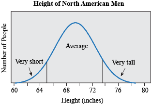
Traits such as height are called quantitative or continuous traits. They are of great importance in various fields such as evolution, agriculture, and medicine. Many of the desired traits in crops or livestock are quantitative traits: sugar content in fruit, crop yield, or milk production are all good examples. In humans, various traits are of a continuous nature such as blood pressure, IQ, and birth weight.
The most important difference between quantitative and Mendelian (qualitative) traits is the number of genes controlling them. Multiple genes govern quantitative traits, each usually having a small effect (so sometimes these traits are known as polygenic; poly = many). However, each of these genes follows the same rules as Mendelian traits. Another important difference between quantitative and qualitative traits is their sensitivity to environmental factors. Let's go back to our height example. Your genes might say you have the potential of growing up to be 71 in., but if you don't have good nutrition while growing up (an environmental effect), you might not reach this height. See, this is why your Mamma is always telling you to eat your veggies! So, in the case of quantitative traits, phenotypic variation (designated VP), is primarily the combination of variation resulting from different sources: variation from genetic effects (designated VG) + variation resulting from environmental effects (designated VE).
VP = VG + VE
Other factors, such as variation resulting from interactions between genetic and environmental effects (designated VGE), are also important in quantitative genetics, but we won't discuss them here.
Because in quantitative traits there is no simple relationship between genotype and phenotype as in qualitative traits, different methods are used to study them. This is when statistics come in handy. Two key statistical parameters to understand the genetics of quantitative traits and pretty much anything in the world are the mean and the variance. The mean, or average, is simply a measure of the middle value in a data set. It is calculated by adding all the values in the set together and then dividing the result by the total number of values (e.g. the average of 2, 5 and 8 is (2+5+8)/3 = 5). In the USA, the average height for men is 69.3 in. If you measured a random man on the street, there is a good chance he would measure close to 69.3 in. The variance describes the spread or variability of a data set by representing how far values lie from the average. If the variance is high, it means many of the values fall far from the mean; on the contrary, if the variance is low, then most values fall really close to the mean. If the variance is 0, then there is no variation at all in the data set: all values are the same.
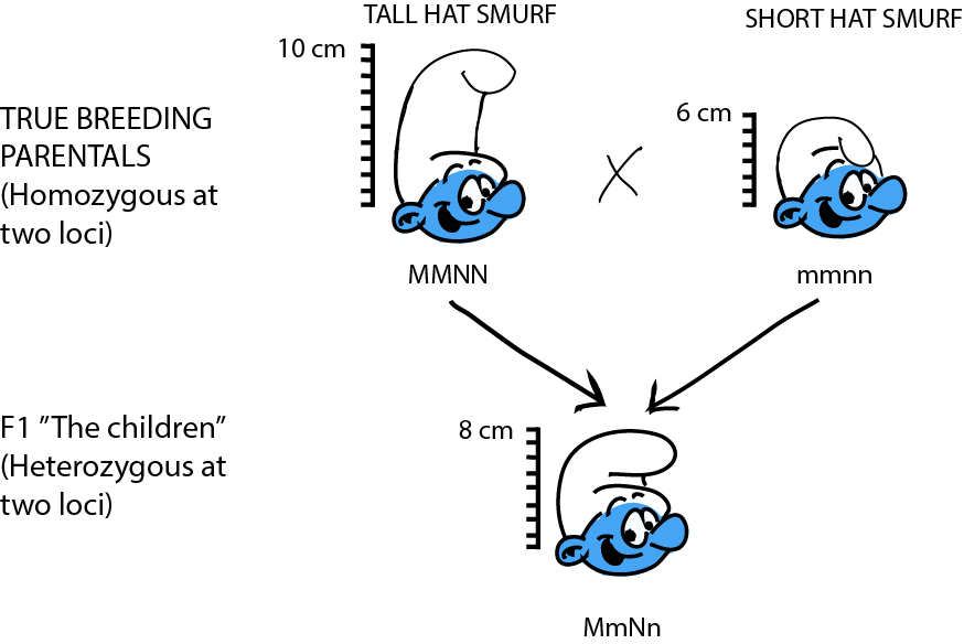
Let's work through a simple, theoretical example to examine the basic genetics of quantitative traits. In Smurfs, hat height is a quantitative trait determined by two loci: M and N, each with two alleles. Sure, hat height doesn't sound very biological, but have you ever seen a Smurf without a hat? As far as we know, it might be organic! At locus M, the allele M contributes 2 inches to hat height, while m only contributes 1 inch. At locus N, allele N contributes 3 inches to the height, while allele n only 2 inches. We cross a group of Smurfs with a genotype MMNN (and thus with an expected phenotype of 2 + 2 + 3 + 3 = 10 in), to a second group of Smurfs with an mmnn genotype (and thus with an expected phenotype 1 + 1 + 2 + 2 = 6 in). The F1, MmNn, fall right in between the parentals (2 + 1 + 3 + 2 = 8 in).
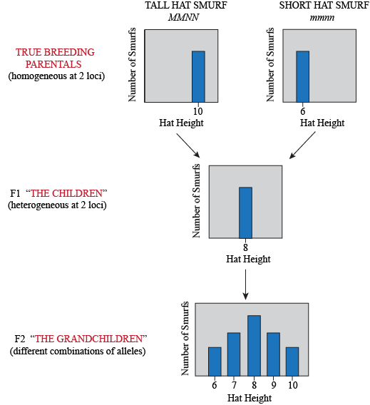
What do the F2 look like? Yet again, the trick to figure this one out is to think about what kind of gametes the F1 produce. Assuming loci M and N are unlinked, then for each we can imagine a bag of marbles. The F1's genotype is MmNn, so in bag M, we have equal quantities of both "M" and "m" marbles; in bag N, we have equal quantities of both "N" and "n" marbles. For each gamete, we draw at random a marble from each bag. So… what are all the possible combinations?
For each individual in the F2 generation, we pick two gametes and combine them. Yeap, lots of possible combinations: 9 of them to be exact, so there are 9 possible genotypes. However, once we add the height value of each allele in each genotype together, we find that these 9 genotypes turn into only 5 phenotypes:
| Genotypes | Phenotype Breakdown | Total Phenotypes |
|---|---|---|
| MMNN | 2 + 2 + 3 + 3 | 10 |
| MMNn | 2 + 2 + 3 + 2 | 9 |
| MMnn | 2 + 2 + 2 + 2 | 8 |
| MmNN | 2 + 1 + 3 + 3 | 9 |
| MmNn | 2 + 1 + 3 + 2 | 8 |
| Mmnn | 2 + 1 + 2 + 2 | 7 |
| mmNN | 1 + 1 + 3 + 3 | 8 |
| mmNn | 1 + 1 + 3 + 2 | 7 |
| mmnn | 1 + 1 + 2 + 2 | 6 |
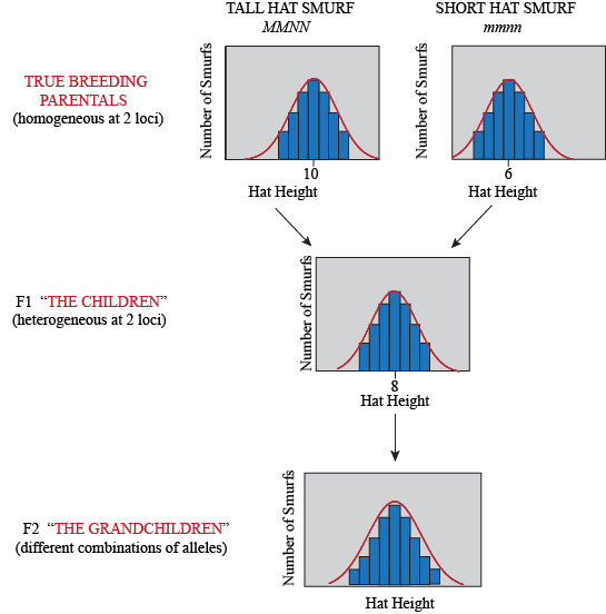
Of course, not only genes determine hat height in Smurfs, but also how many smurfberries they ate during childhood (an environmental factor). So even Smurfs with the same genotype will have some differences in their phenotype, depending on what they've been eating. Here is what our experiment looks like when we consider environmental variation:
Our Smurf hat height example involves only two loci with two alleles each. As you add more loci, the story gets much more complicated rather fast…
| Number of Loci | Number of Alleles | Number of Genotypes in the F2 | Number of Phenotypes in the F2 |
|---|---|---|---|
| 1 | 2 | 3 | 3 |
| 2 | 4 | 9 | 5 |
| 3 | 6 | 27 | 7 |
| 4 | 8 | 81 | 9 |
| 5 | 10 | 243 | 11 |
| 10 | 20 | 59, 049 | 21 |
| n | 2n | (3)n | 2n + 1 |
Additive genetic variance (VA): potentially the most important type of gene action in quantitative traits. In this type of genetic variation, each allele adds a specific value to the phenotype. Our Smurf hat height example above assumed additive variation. In a way, it is like adding cash: each of the coins you found in your pants pocket is an allele, and each adds a value to your piggy bank. So if you found two quarters, a dime and three nickels, your previously empty piggy bank has now a cash "phenotype" of 75 cents.
Dominance genetic variance (VD): in this case, we have the same relationship between alleles at a single locus as we discussed in classical Mendelian inheritance. Homozygous dominant and heterozygous genotypes contribute the same amount to the phenotype (effect of MM = effect of Mm). The effect of the recessive allele is "hidden" in heterozygotes (Mm) and is only seen when homozygous (mm). Let's modify our Smurf hat height example to reflect only dominant genetic variation. At locus M, the allele M is dominant and contributes 2 inches, while m is recessive and contributes only 1 inch. At locus N, allele N is dominant and contributes 3 inches, while allele n is recessive and contributes 2 inches. Now an individual whose genotype is MMNN has an expected phenotype of 2 + 3 = 5 in, while under the additive variation model it was 10 in (2 + 2 + 3 + 3 = 10 in, as each allele individually contributes a value). Our second group of Smurfs, mmnn, now has an expected phenotype of 1 + 2 = 3 in. Under the additive variation model, this same genotype had an expected phenotype 1 + 1 + 2 + 2 = 6 in. Now, in the F1, MmNn, the expected phenotype is 2 + 3 = 5 in, as only the presence of the dominant alleles contributes to the height of the hat. Compare to its expected value under the additive variation model: 2 + 1 + 3 + 2 = 8 in.
Epistatic variance or interaction genetic variance (VI): In this case, there is an interaction between different loci affecting a trait. By "interaction" we mean usually an effect on the phenotype beyond additive. Let's go back to the Smurf hat example. Instead of an additive gene action at the loci M and N, let's assume they have an epistatic interaction when alleles M and N are present: instead of simply adding up their values, when alleles M and NM are present, the hat will also double in height. So, our new phenotypic values are as follows: MMNN: 2(2 + 2 + 3 + 3) = 20 in; mmnn 1 + 1 + 2 + 2 = 6 in (no change as allele M and N are absent); MmNn 2(2 + 1 + 3 + 2) = 16 in. If we also look at some F2 phenotypes, MmnnM is 2 + 1 + 2 + 2 = 7 in (no epistatic effect as allele N is absent), but in MMNn, we see it again: 2(2 +2 + 3 + 2)= 18 in.
So that the full, expanded equation to calculate the phenotype variance is:
VP = (VA + VD + VI) + VE
A real trait, unlike our Smurf hat height example, will likely have many loci reflecting a combination of additive, dominant, and epistatic interactions that, as you might imagine, make their study rather complicated. In fact, we know very little about the actual genes behind quantitative traits. Scientists most often study them through "quantitative trait loci" (QTL) analysis. Through this method, it is possible to identify regions of the genome affecting a quantitative trait and how they interact with one another (additively, epistatically, and so on). These regions, however, are often really large and contain hundreds of genes. Nevertheless, using this method and related techniques, scientists have identified single genes affecting weight in tomatoes, pigmentation in fruit flies, and loss of pelvic fins in sticklebacks. For no single quantitative trait in any species, however, do we have a complete understanding of its determination: identifying all the genes involved, their interactions, and the contribution of the environment is one of the frontiers in genetic research.
Heritability
Heritability represents the proportion of the phenotypic variation in a population that is explained by genetic factors (and as a proportion, it is a number between 0 and 1, with 0 meaning "none" and 1 meaning "all"). Heritability is useful for estimating the relative contribution of genetic and environmental factors to a particular trait. For example, how is intelligence in people determined? Did someone with a high IQ just inherit it from her parents, or does stimulation while growing up make a difference too?Broad sense heritability (H2) is the ratio of the total genetic variance to total phenotypic variance:
H2 = VG/VP
Thus, the broad sense heritability includes additive, dominant, and possible epistatic effects since, remember, VG is a combination of all those things.
As it turns out, IQ and most other human complex traits seem to have both a genetic and an environmental component. What researchers can't agree on, though, is how much each one contributes. Studies suggest the heritability of IQ ranges somewhere between 40 to 80%. So at one end of the range (40%) genes play a small role, and mostly the environment defines someone's IQ. On the other hand, at the other end of the range (80%), IQ would be determined almost entirely by a person's genotype.
Narrow sense heritability is the ratio of only the additive genetic variance to the total phenotypic variance:
h2 = VA/VP
Why distinguish between the two types of heritability? The narrow sense heritability is important because both artificial and natural selection act primarily on additive genetic variation. When an individual reproduces, it passes along individual alleles, not specific combinations. So dominance and epistatic genetic variance are not passed along to offspring with the values they had in the parents, as the allele combinations responsible for them are broken down. For example, in the case of dominance variance, parents carrying various dominant alleles might also be hiding some recessive ones; they could be heterozygous. So while the parents' phenotype reflects the effect of the dominant alleles, the offspring could inherit a combination of their recessive alleles and look completely different. Additive components, however, are inherited as is: the value of additive alleles in the parents is the same in the offspring regardless of the shuffling. Therefore, additive genetic variance is usually responsible for similarities among relatives (assuming there's no common environmental cause!) and allows us to predict the phenotype of an offspring.
Brain Snacks
- We are Siamese, if you please: The Siamese coat color (pale body, dark "points") in cats is a great example of how the environment affects gene expression – only the cool extremities of the body can make melanin, which gives the dark coloration. A mutation in one of the genes involved in melanin production makes it temperature sensitive, so it no longer works in warmer parts of the body, leading to a pale coat color in those areas. So, technically speaking, if you took a Siamese cat somewhere very cold, it would turn completely dark brown!
- Seeing Double! Studying quantitative traits in humans is very tricky, but one of the best ways to look at how genes and the environment interact is by carrying out twin studies. There are two types of twins: monozygous (identical twins with identical genes) and dizygous (non-identical, or fraternal, twins who only share 50% of their DNA). Because twins usually share the same environment when they're growing up, you can use differences in expression rates between identical and non-identical twins to figure out which has the biggest influence: nature or nurture.