Using Roots to Construct Rough Graphs of Polynomials at a Glance

We're trekking right up Polynomial Mountain with our guides, the polynomials. What are those crazy little guys doing now? It looks like they're all drawing squiggly lines in the sand.

Wait. Are they writing their names or drawing a picture of themselves? That's it. When we look carefully, we see that they've used their roots to draw self-portraits in the sand. We can even see patterns based on their degree.

Could we use what we've discovered on the planet of polynomials to make our own sketches of our polynomial friends?

Yes. We think we're ready to construct some rough sketches of these guys. From our previous visit to this planet, we already know how to graph first- and second-degree polynomials (a.k.a. linear and quadratic functions). Now we'll look at how to use their roots to construct rough graphs of higher-order polynomials. We can use the Remainder Theorem to check for roots, and then use synthetic division and factoring to find the rest.

Let's ask our alien friends for some of their little tricks and hints to make this easy.

First, the roots, also called the zeros, of our polynomials are the points where they cross the x-axis.

Second, we can have a general idea what our graph will look like based on the degree of the polynomial.

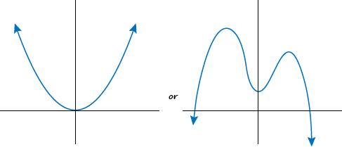
The two ends of an even-degree polynomial graph as either "up" on both ends or "down" on both ends. Like this:

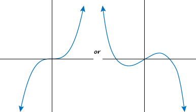
Odd-degree polynomials graph with one end "up" and one end "down."

We call all this a polynomial's end behavior. Polynomials don't see any difference between front-end behavior and rear-end behavior, which explains why they can be so hard to get along with sometimes.

The last hint we have as to the shape of our graph is the degree of the polynomial. The hint has an official name, the Turning Point Theorem, but we don't need to worry about that.

The basic idea is that a graph always has fewer turning points than its polynomial's degree.

The graph of a second-degree polynomial has at most 1 turn, while a third-degree polynomial has at most 2 turns. A turning point is a spot where the polynomial changes direction (moving up or down).

The best way to see how this all plays out is to actually start making a graph.

Sample Problem

Graph y = x³ – 7x + 6.

First we'll find possible roots by looking at the factors of the constant 6. They are x = ±6, ±3, ±2, and ±1. Nothing could be simpler than plugging in a 1, so we'll do that first.

P(1) = (1)³ – 7(1) + 6

= 1 – 7 + 6

= 0

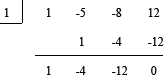
Whether it's efficiency or laziness, we won't argue with results: we know that x – 1 must be a factor of our polynomial, and one of its roots is x = 1. Now we use this 1 in our synthetic division to find all the factors of the polynomial.

The second factor is x² + x – 6. Factoring again gives us (x + 3)(x – 2). Mix all our factors together to find the roots.

P(x) = (x – 1)(x + 3)(x – 2)

Setting each part equal to zero gives us roots of x = 1, -3, and 2. That means the points (1, 0), (-3, 0), and (2, 0) all show up on our graph.

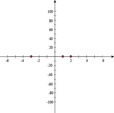
Notice that the graph must touch the x-axis at these three points, and possibly cross over. Not in a "now we're dead" sense, but in a "now our sign is the opposite" one.

Our polynomial has degree 3 (because of x³), and this is odd. Not unusual; just odd. Its end behavior will have one end pointing up and one end pointing down.

We'll need at least one more point in each section of the graph to get the general shape. What are the sections? There's one on each side of each root.

We'll just pick a few x-values, each one from a different section of the graph.

P(-5) = (-5)³ – 7(-5) + 6 = -84 → (-5, -84)

P(0) = (0)³ – 7(0) + 6 = 6 → (0, 6)

P(1.5) = (1.5)³ – 7(1.5) + 6 = -1.125 → (1.5, -1.125)

P(5) = (5)³ – 7(5) + 6 = 96 → (5, 96)

Now we have enough points to get a rough graph of our polynomial, by plotting these additional four points and connecting them with a smooth curve. We can afford to be a bit loosey-goosey with our drawing. We just want to get the overall behavior of the polynomial.

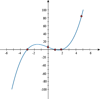
Now we can see that the graphs turns twice, between x = -3 and 1, and between x = 1 and 2. This beautiful graph turns points and heads.

Sample Problem

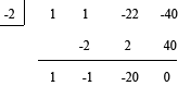
Graph f(x) = x³ + x² – 22x – 40.

The first rule of graphing polynomials is, "Don't talk about graphing polynomials." Whoops, we already broke that one. The second rule is, "Find possible roots by looking at the factors of the constant." Following one out of two rules isn't that bad, right?

The factors of 40 are ±40, ±20, ±10, ±8, ±5, ±4, ±2 and ±1. That's a lot of factors. Dig in.

f(1) = (1)³ + (1)² – 22(1) – 40

= 1 + 1 – 62

= -60

Nope, that isn't a factor. Plugging in -1 wouldn't improve things much, either. Let's try 2.

f(2) = (2)³ + (2)² – 22(2) – 40

= 8 + 4 – 44 – 40

= -72

Swing and a miss. Maybe -2?

f(-2) = (-2)³ + (-2)² – 22(-2) – 40

= -8 + 4 + 44 – 40

= 0

Ding, ding, ding, we have a winner. Our first root is x = -2, so our first factor is x + 2.

We run that -2 through a round of synthetic division to find our other roots.

Our polynomial is:

f(x) = (x + 2)(x² – x – 20)

This factors further to:

f(x) = (x + 2)(x + 4)(x – 5)

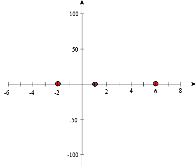
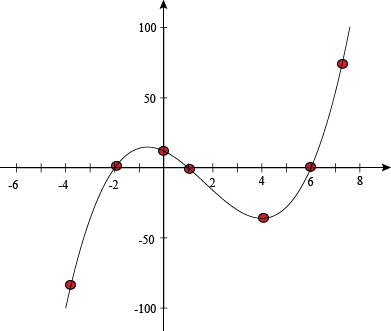
Our roots, ladies and gents: x = -2, -4, and 5. Give them a round of applause as they take their spots on the graph.

We need more points, though. We'll pick a few more x-values to try, one from each section. Other numbers would work, but we want to keep the numbers small and manageable.

f(-5) = (-5)³ + (-5)² – 22(-5) – 40 = -30 → (-5, -30)

f(-3) = (-3)³ + (-3)² – 22(-3) – 40 = 8 → (-3, 8)

f(0) = (0)³ + (0)² – 22(0) – 40 = -40 → (0, -40)

f(6) = (6)³ + (6)² – 22(6) – 40 = 80 → (6, 80)

Now we have enough points to get a rough graph of our polynomial. We'll need even more points if we want to make the leaderboards, though.

The degree of the polynomial is odd, so it will have the two ends pointing in opposite directions.

That's an award-winning graph right there. For what award, we're not sure. Maybe the Most Recent Graph Award.

That isn't really a ringing endorsement, is it? Let's try another one.

Sample Problem

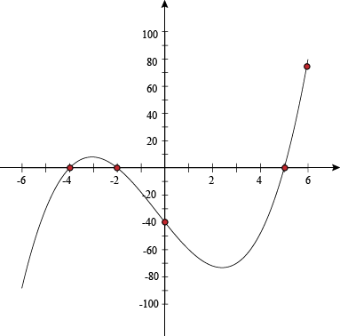
Graph y = x⁵.

Um, we think we found a zero already. It's zero.

P(0) = (0)⁵ = 0

The degree, 5, is odd, so we know the end behavior has one end "up" and the other "down." It's everything in the middle that's kind of hazy.

We don't have any nice sections to choose points from, so we'll make a table and calculate several values to get our ordered pairs.

Three numbers in each direction should be enough to have a rough idea of what the graph looks like, and a rough idea is all we need.

Okay, that was our third odd graph in a row. We need to switch things up, and then we'll blow this popsicle stand.

Sample Problem

Graph f(x) = x⁴ – 9x².

With all the use we've gotten out of the Remainder Theorem to find factors and roots, we can forget that sometimes it's easier to just factor the polynomial directly.

x⁴ – 9x² = 0

x²(x² – 9) = 0

Our roots here are x = 0 and x = ± 3. See? Simple. Don't work for the math if you can avoid it. Make the math work for you.

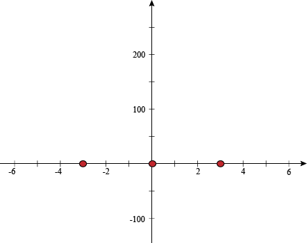
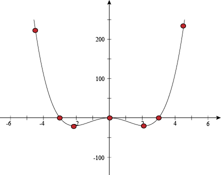
Even-degree polynomials have end behavior where the ends both point up or both point down. Its degree is 4, so can have no more than 3 turns. Also, this is the last problem of the section, and we're tired, so it can't be too hard. We just need to find a few more points. Let's slice it up into sections again, and find one point between each of those roots.

P(-5) = (-5)⁴ – 9(-5)² = 400 → (-5, 400)

P(-2) = (-2)⁴ – 9(-2)² = -20 → (-2, -20)

P(2) = (2)⁴ – 9(2)² = -20 → (2, -20)

P(5) = (5)⁴ – 9(5)² = 400 → (-5, 400)

Wait, we could've plotted x = ±1 and ±4, and the numbers wouldn't have been as hard. That's what happens when graphing while tired, we suppose. That, and graphs that look suspiciously like beds, and sheep, and pillows.